QORE — the engine behind every chemistry.
QpiVolta Optimization and Research Engine — a closed-loop computational + robotic platform that screens, synthesizes and validates novel materials across ten technology domains, at thousands-per-week throughput.
One discovery engine. Ten domains.
QORE is general-purpose — pre-trained on millions of structures, fine-tuned per target class. Battery materials are how we proved it. The same loop applies anywhere a new material is needed.
- 01Catalysts
- 02Polymers
- 03Coatings
- 04Battery materials
- 05Photovoltaics
- 06Alloys
- 07Carbon capture
- 08Hydrogen storage
- 09Additives
- 10Semiconductors
Five engines. One workflow.
QORE is the application layer of the discovery stack. Specialists for simulation, generation, mining, language reasoning over chemistry, and autonomous lab orchestration — all running against the same shared infrastructure.
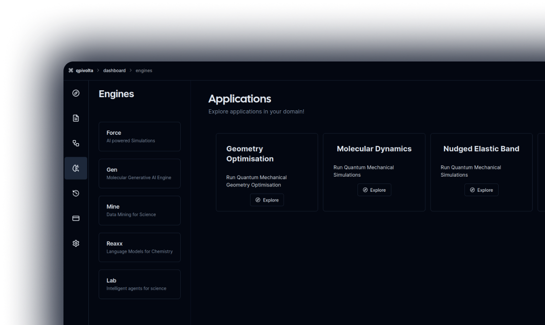
- 01ForceAI-powered simulations
- 02GenMolecular generative AI engine
- 03MineData mining for science
- 04ReaxxLanguage models for chemistry
- 05LabIntelligent agents for science
The space of inorganic compositions is too large to search directly.
We start from the known: millions of crystal structures, projected to two dimensions so the territory can be navigated before it's searched.
Each point is a known structure.
4.2M structures, embedded by a graph encoder. Distance corresponds to structural similarity.
Structural families cluster.
Similar frameworks land near each other. The grouping comes from the geometry, not from labels.
We focus on one cluster.
The rest of the pipeline operates within it.
Within one cluster, 40 phase spaces are searched in parallel.
A custom interatomic forcefield, trained on QpiVolta data and calibrated against DFT, sweeps each composition space roughly 1000× faster than first-principles — so many can run concurrently.
Phase spaces, side by side.
Each hex is one chemistry. The interior is its composition triangle, gridded by ratio.
The forcefield drives the search.
Calibrated against DFT, ~1000× faster. The marginal cost of an extra sample drops to near-zero.
40 in parallel. Hot pockets surface.
A few chemistries show clear minima; most stay flat. Compute is reallocated overnight toward what's converging.
A foundation model proposes stoichiometries.
Pre-trained on the structural corpus, fine-tuned on QpiVolta targets. The periodic table lights up by usage frequency as proposals are drawn.
Lithium dominates.
Nearly every proposal contains it. The model is conditioned on our target class.
Partner elements surface.
A handful dominate. These were not specified — the model selected them from the corpus.
Dark cells are open questions.
Some are physically excluded; others are under-represented in training. Priors are updated nightly.
Where does the next batch of compute and bench time go?
A Bayesian acquisition function selects each next batch. The posterior sharpens with every iteration.
Broad prior.
Several regions look comparable. The model has not yet differentiated them.
The posterior sharpens.
Dead regions drop off. Live ones attract samples.
Converged.
One region dominates. The next batch is allocated there.
From a million proposals to a few real cells, in five gates.
Each gate is a different filter, applied by a different tool. ~1M proposals per day, ~12 cells retained per year.
~1M proposals / day.
Generated continuously by the foundation model. Most are filtered out at the next gate.
Physics removes 99.7%.
Anything that fails simulation does not reach synthesis.
~12 retained / year.
Surviving cells pass DFT screening, synthesis, measurement, and cycling.
For each target, a synthesis route is planned.
A retrosynthesis model plans a viable route from precursors we can source. Tree search over disconnections; the highlighted path is the selected route.
Start at the target.
Root of the search tree. The model evaluates disconnections that simplify assembly.
Branches expand.
Node size is search effort; opacity is predicted value. Larger nodes received more rollouts.
One path is selected.
Short route, available reagents. Cost and predicted yield are reported alongside it.
The high-throughput lab synthesizes survivors overnight.
Cleanrooms operate unattended. Every wafer is tagged and traceable to the proposal that produced it. Telemetry below is live.
Furnace at setpoint.
Closed-loop control. Settles to within 2°C in under 2 minutes.
Sealed atmosphere.
Sensitive chemistries remain inert end-to-end. Pressure variance held below 1%.
Wafers per hour, unattended.
Vision-based QC, lot-traceable, archived.
The model predicts conductivity. Physics validates it.
A full cell model runs against each candidate before the bench does, predicting the measurement before it is taken.
Full charge.
SoC at 100%. Voltage at the upper plateau.
Discharge.
Lithium concentration migrates across the stack. Heat localises at the interface.
Model vs. bench.
Simulated discharge curve overlays the measured one within 1%.
108 virtual cells, cycled in parallel.
A single simulation indicates whether a cell works. 108 simulations identify which microstructure continues to work. Each tile is a full cycling run.
Many cells, cycling.
Same chemistry, different microstructures. The grid starts identical and diverges from cycle one.
Weak geometries fail.
Mid-life, the plating front accumulates. Capacity collapses. Tiles drop out.
The survivor wins.
By end of run, one geometry remains on its linear curve. That recipe is queued for the bench.
AI agents coordinate the full workflow.
Each stage runs a specialist model. A meta-agent schedules tasks across them. Humans set targets; the pipeline runs continuously.
One agent per stage.
Specialists for proposal, acquisition, routing, lab ops, physics, and retraining.
A meta-agent coordinates.
Tasks transition between agents continuously. Failures route back to retraining; successes queue for synthesis.
The loop runs continuously.
Targets are re-prioritised overnight. Each morning, the queue reflects the latest results.